A primer on economic growth

Everything you need to know about what fuels the engine

Why are some countries rich and some poor? Why did growth only take off around the 18th century? Why is North Korea growing faster than Canada? To meet the demand for the burgeoning interest in economic growth, and also to refine my own thinking on this topic, I have decided to write an undergraduate-level primer on the topic.

Ultimately, I believe that teaching economics is amongst the most invaluable functions of the discipline. If you can communicate your knowledge to the outside world, and clarify it to be comprehensible to an educated layman, you know you have fully mastered a topic. Most importantly, for economics to disseminate across the generations, and to preserve or justify its existence, we need a mechanism for it to spread, and that is teaching it. Why would we produce economics if not to inform others: for instance via policy advice, understanding human interaction better, or helping firms make better forecasts and decisions, and so on?

As this is for pedagogical purposes, unlike in my other posts, I assume only the bare minimum of economics knowledge (Econ 101 level). I will however work with a high-school level background in (multivariate) calculus [1]. I will start with an overview of the (in)famous Solow model, which will be a building block to the more realistic endogenous growth models that constitute the main building blocks of this primer.

Solow

In this model, the factors of production are K=capital [2] and L=labour. We will use a production function to describe how those inputs create Y=output, applied to the entire economy. This aggregate production function, as they are known, will satisfy the following properties:

1. Constant returns to scale. Output scales linearly with input. Double the quantity of inputs, and output will also double, and so on. In the technical jargon, we can say that such a function is homogenous of degree one.

2. Diminishing marginal returns. The second derivative of output with respect to an input is negative, whilst its first derivative is positive. Intuitively, with a constant labour force, each new factory necessarily makes a smaller contribution to output, and vice-versa.

3. Inada conditions: as the quantity of an input tends to infinity, the first derivative of output with respect to that input approaches zero. This follows naturally from (2).

Let Y = AK^αL^(1-α) [3], where A represents total-factor productivity or technology (for now a constant residual), and the capital elasticity α is between 0 and 1. Population grows at a constant rate g, so L’ = (1+g)L is our labour stock in the next period. Capital accumulation is described as:

K’ = (1-δ)K + I,

I = sY

where δ is the constant depreciation rate of the capital stock. I=investment=S=savings, where each household saves a fraction s of its income, so sY gives total savings. In this model, there are no open economies nor governments (taxes or government spending) nor money. Hence, saving is simply the proportion of income=output that is not used for consumption today. Financial markets are fully efficient, no one hides money under their mattress [4], so all savings finance investment: spending on new additions to the capital stock. Note that capital is simply the set of goods used to produce other goods. Human capital comes later, but for now that goes in A, so K is restricted to physical capital.

Output per worker (so GDP per capita = living standards, see here for my defence of GDP) follows easily. I will assume that everyone is a participant in the labour force:

y = Y/L = AK^αL^(1-α)/L = A(K/L)^α = Ak^α

for k = capital per worker. So in this model, living standards are determined by capital.

Capital accumulation per worker is given by:

K’/L = [(1-δ)K+sY]/L,

(K’/L’)(L’/L) = (1-δ)k + sy

(1+g)k’ = (1-δ)k + sAk^α

therefore k’ = [(1-δ)k + sAk^α]/(1+g)

Now I must draw everyone's attention to this diagram (substitute N for L):

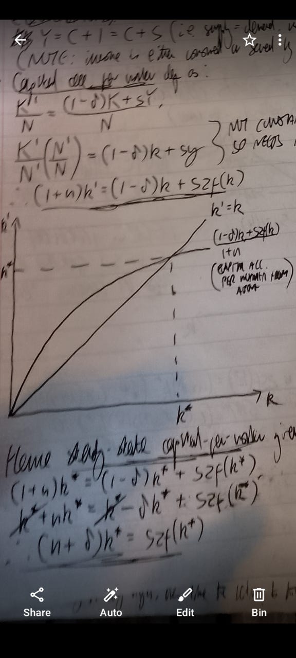
As you can see, the graph of capital accumulation per worker is concave in k, which follows naturally from diminishing marginal returns. Eventually, the returns of new capital additions will be dwarfed by capital depreciation, so a steady-state arises. The equation for that steady-state is given in the above diagram. Intuitively, the LHS represents the investment per worker needed to maintain the existing capital stock over time, and the RHS is investment per worker. In the steady-state, each worker invests just as much as is required to maintain the capital stock.

Now let us consider the implications for living standards with another diagram:

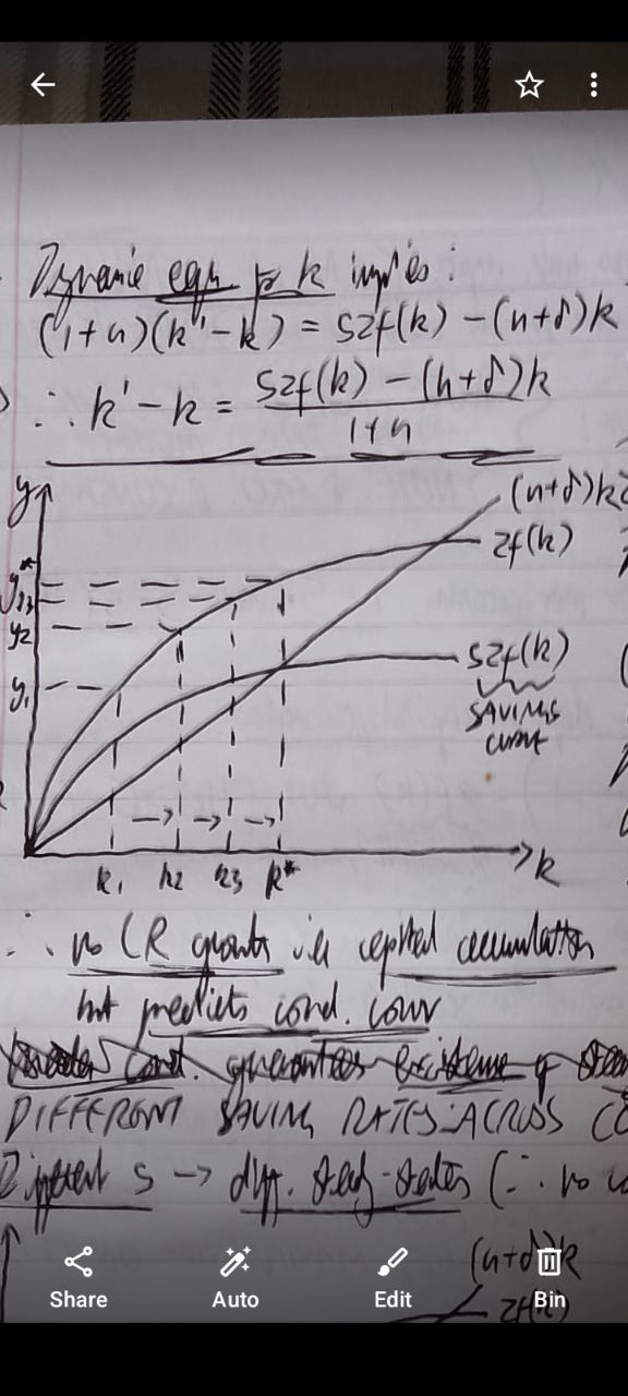
In this case, capital accumulation, determined by savings per worker, occurs at a declining positive rate, as one would expect from diminishing returns. Eventually, at the stage where new additions are outweighed by depreciation, the steady-state for capital will be reached, which implies a steady-state for GDP per capita.

As such, the main result arises. Capital alone cannot produce a sustained and permanent rise in living standards. Even raising the saving rate will only generate a rise in steady-state GDP per capita - perhaps best exemplified by China in recent times, which relies heavily on capital accumulation in its development model. Here is a perfect example of how an unrealistic model can produce a profound insight into how the world works. Hence, to explain the phenomenon of economic growth, we must look elsewhere.

Technological progress

By taking partial derivatives of the Solow production function with respect to K or L, you can clearly see that both are subject to diminishing marginal returns. Both marginal products are a function of capital per worker, technology, and their respective elasticities. Only capital per worker is endogenous (explained by the model) here, and that is the term that abides by diminishing returns. Yet diminishing marginal returns to factors of production IS the reason for the core result, that all growth is simply a temporary convergence to a steady-state and that sustained and permanent growth is impossible. Hence, to overcome this feature, it seems sensible to pivot our focus to the elasticities or technology.

Start with the elasticities. Even if the capital and labour elasticities differ, the model imposes constant returns to scale: the restriction that both must sum to one. As such, whilst changing their elasticities will change the respective contributions of capital and labour, and their shares of output, this exercise will bear no implications on our primary conclusion.

We are now left with the elephant in the room, which until now I have been deliberately ignoring: technology. In the Solow model, such is treated as a residual. However, as Lucas demonstrated, TFP may be the most important of all in accounting for the gargantuan cross-country discrepancies in wealth or growth.

Another core prediction of the Solow model is that, conditional on two countries having an identical saving rate, over time the poorer country will catch up to the richer one. In other words, the poorer grows faster than the richer nation. This result is known as conditional convergence. As is obvious from the model, the poorer country will display higher returns to capital, so investment will flow from richer to poorer countries. Yet empricially, as you can see in Lucas' famous paper, these predictions do not square with reality. Therefore the Solow model is wrong. Furthermore, when economists estimate the value of the total capital stock of each nation, in tandem with the labour force numbers, they always find a substantial proportion of output only accounted for by the residual. To explain why empirical reality contradicts the Solow model, we must gear our attention to technology.

AK model

Our next step will be to isolate the effects of technology in our model, to see whether this residual can generate sustained and permanent growth. To do this, we have a clever trick! Simply set the capital elasticity to one.

When α=1, Y=AK, and δY/δK=A. The marginal product of capital is now a constant, a function of technology, with no diminishing marginal returns whatsoever. GDP per capita as a function of capital per worker also now lacks diminishing returns, as y=Ak. Graphically, we can see the implications clearly:

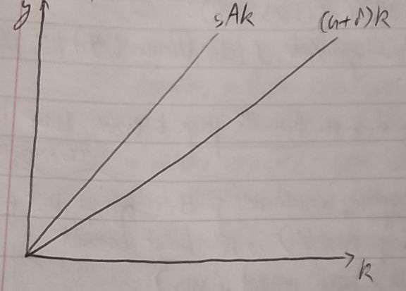
So long as sA > n+δ (almost guaranteed as the right-hand side of this inequality is virtually always a single digit decimal!), we can produce a permanent rise in living standards. There is no steady-state, nor conditional convergence, nor diminishing marginal returns. Our answer lies in technological progress.

Nonetheless, for three immediately obvious reasons, the picture is still incomplete:

1. To obtain these results under the Solow framework, we had to set the capital elasticity to one. Empricially, if this was the case, then labour would yield no share of output. The marginal product of labour would be zero, so no one would be paid anything. Only owners of capital would accrue substantial material gains; a Marxist caricature of how the economy works. Maybe under the most extreme predictions of the AI singularity, this could hold, but certainly right now this is an obviously absurd claim!

2. The AK model implies that growth in living standards is linear, as you can see graphically. In fact, growth is exponential, so this massively understates the extent to which growth is possible.

3. Technology is left as a residual constant here. For a discipline that revolves around analysing the causes of prosperity, we obviously want to explain what drives the main determinant of growth. This is only possible if we treat technological progress as an explicit variable, not just a constant residual. In technical jargon, we want to endogenise the term.

The rest of this post will be devoted to precisely that task. Models that endogenise technological progress are known (conveniently) as endogenous growth models. I hope to demonstrate that, under this approach, a much more realistic approach to analysing growth is possible, despite the recent claims of the “heterodox”.

An introduction to human capital

Mankiw, Romer, and Weil (1992) start with a modification to the conventional Solow model. Technology, rather than scaling the entire function, acts as a complement to labour. In this sense, technology drives growth via its effects on human capital or labour productivity, and in the model is assumed to grow at an exogenous rate γ [5].

Let Y = K^α(AL)^(1-α). Now let y and k be output and capital per effective unit of labour respectively.

y = Y/(AL) = k^α, so again, living standards are driven by capital per worker, with technology as a complement. AL grows at g+γ, whilst the dynamics of k are governed by:

k’ = sy - (g+γ+δ)k = sk^α - (g+γ+δ)k

which implies a steady state of:

k* = [(g+γ+δ-1)/s]^(1/(α-1)).

However, as is clear by substituting this into our production function, this steady state produces long-term growth:

y* = Y/AL = [(g+γ+δ)/s]^(α/(α-1)),

Y/L = A[(g+γ+δ)/s]^(α/(α-1)).

By taking logs, we can also see that this growth is exponential:

ln(Y/L) = lnA + (α/(α-1))[ln(g+γ+δ)-lns],

lnY = ln(AL) + (α/(α-1))[ln(g+γ+δ)-lns],

dlnY/dt = (g + γ)/AL via the chain rule, as AL is the endogenous variable growing at a constant rate g+γ, and the other terms are constant. Therefore…

dY/dt = (dlnY/dt)(dY/dlnY) = (g+γ)Y/AL = (g+γ)k^α, which grows exponentially.

Calibrating the equation for lnY using OLS, assuming that γ does not differ via country (given diffusion of ideas and technology across borders: more on this later!), and neither does δ, and ln(AL) includes country-specific factors such as climate, institutions and so on, we get the following. The authors find that saving and population growth affects economic growth in the signs that Solow predicts, yet not in the magnitudes. There is still a large proportion of growth unaccounted for. See the paper for more on this.

However, an augmented model that incorporates human capital as a distinct endogenous variable does predict the magnitudes well. Using the usual Cobb-Douglas assumptions, let…

Y = K^αH^β(AL)^(1-α-β). Notice that technology still augments labour productivity. Indeed, the authors are unclear in what separates A from H. I take human capital to mean the intangible factors of production that are person-specific (their own talent or effort, acquired skills and knowledge, and so on - distinct from general technologies or production processes that are economy-wide), though if my definition is wrong, I am happy to be corrected. Notice too that human capital still abides by diminishing returns here. In later models, this assumption becomes less relevant. Output per unit of effective labour follows; its equation is rather clunky so I will leave this as an exercise for the reader. Just note that y is now a function of human capital too.

Also let sk be the fraction of savings per worker allocated to physical capital, and sh the fraction devoted to human capital. Human and physical capital depreciate at the same rate (again controversial: more later!). The dynamics for both types of capital are the same as before, with their respective fractions of saving. From there, their steady-states can be derived, which also generate long-run exponential growth; more closely matching the empirical data.

Endogenous growth with increasing returns

Nonetheless, the augmented Solow model, whilst matching the data well, still retains the assumption of diminishing marginal returns to the factors of production. Suppose we want to eradicate this assumption altogether. That is precisely what Romer (1986), pioneering endogenous growth theory, does. Colloquially, this model is known as the learning-by-doing model.

Here, the key intuition is that knowledge can be accumulated during the production process itself. Whilst there may be diminishing marginal returns to physical capital, when a firm invests in technology or skills, other firms learn from this process. In other words, knowledge and innovation is nonrival [6]. Hence, we should expect positive spillovers from ideas or technologies, which in aggregate eliminates the diminishing returns to investment (capital accumulation) at the firm-level. In practice, investment into physical capital comes with it investment into (often new or more efficient) production processes, with the respective adaptations to skills and new technologies required. A microfounded model, using a representative firm’s production function rather than an aggregate one, also arises: resolving the objections raised in the Cambridge capital controversies, and the Lucas critique. I will now present a simplified introduction to this model.

For a representative firm i, let Yi = Ki^α(βLi)^(1-α), where β represents economy-wide knowledge or technology. Here, β = λK, where λ>0 captures the positive spillover effects of capital accumulation. At the macro level, the following results:

Y = K^α(λKL)^(1-α) = K(λL)^(1-α)

so diminishing returns dissipate in aggregate, whilst labour is complemented as in the augmented Solow model.

Capital accumulation is given by K’ = sY + (1-δ)K, and holding population growth constant, this becomes k' = sk(λL)^(1-α) + (1-δ)k per worker. This grows at a constant rate:

(k’-k)/k = s(λL)^(1-α) - δ

which produces identical dynamics to the AK model, with the corresponding implications.

The primary innovation in these results are scale effects. The rate of growth is not only a function of savings or spillover effects, but of an aggregate variable L. Intuitively, a larger labour force generates a higher growth rate of capital per worker, hence a higher growth rate of output. Intuitively, a larger population implies more geniuses, and greater production of ideas, which diffuse across the economy given the positive spillovers. Hence the model can incorporate increasing returns to scale: a major departure from Cobb-Douglas.

Alternatively, with β = λk you get:

Y = K^α(λkL)^(1-α) = K^α(λK)^(1-α) = λ^(1-α)K,

(k’-k)/k = sλ^(1-α) - δ

which recovers constant returns to scale. Likewise, the relationship between technology and capital may also be nonlinear, which would bear implications for the dynamics of growth predicted. In this sense, the theory arguably raises more questions than answers, and is consistent with a wide range of modelling approaches. If your prior is that past scientific and technological advancements provide the basis for future innovation (somewhat analogous to the Whig model of history), and that even incremental improvements to the status quo can generate exponential returns (as is the case with Moore's Law), then you may advocate for increasing returns to scale. However, there is far more discussion on the Gordon hypothesis, that as you achieve the “low-hanging fruit”, then future discovery becomes much harder.

Personally, I think the Gordon hypothesis was a convincing account for the slowdown of the 2010s, yet especially with the advent of AGI cannot hold over a much wider timeline. If AGI, and the prior work integral to its development, is not a textbook example of increasing returns from existing capital, then I don't know what is! I actually think that scale may be an underrated factor as to why growth is poor in Britain: an outflow of venture capital, scientists, startups and the like to America, to take advantage of the agglomeration effects resulting from spillovers there. Clearly, there are nonlinearities in progress, which is what makes growth so hard to model.

In my view, the fact that such a theory can incorporate a wide variety of predictions places doubt on its falsifiability. Nonetheless, this was the first attempt to depart from a zero growth steady-state, so the model still deserves an immense degree of credit. Indeed, the positive spillovers from this paper spurned an entire subfield of economics!

Modelling the dynamics of human capital

An alternative approach to endogenous growth, proposed by Lucas (1988), excludes physical capital altogether - pivoting its approach towards human capital. Indeed, this is the first model to incorporate human capital explicitly as a distinct variable, and goes further than Mankiw, Romer and Weil (1992): it endogenises both the returns and costs to human capital accumulation, on its supply-side (households) and demand-side (firms). What follows is a highly simplified version of this model, which still encaptures its main lessons.

For a representative household, consumption satisfies the following budget constraint:

C = ωuHs

where ω is the real wage, u is the fraction of time spent working, and Hs is the household’s supply of human capital (uHs is equivalent to labour supply here). Each household either utilises its existing human capital stock in the labour market, or spends time acquiring new human capital (via training or education). There is no leisure in this model. Hence:

H's = b(1-u)Hs

where b represents the returns to investing existing human capital into acquiring additional capital.

On the firm-side, Y = AuHd, where Hd is the firm’s demand for human capital. Profits are given by:

Π = Y - ωuHd = (A-ω)uHd

where A is a constant residual as in the Solow model; in this case the marginal product of labour (as for L = uHs = uHd in equilibrium, δY/δL = A). Solving for the FOC for profit-maximisation gives A=ω, as is standard.

Hence, in equilibrium (for Hs=Hd=H), C = AuH = Y, with the growth rate of H given by b(1-u) - 1. So long as b(1-u)>1, human capital will grow endogenously at a constant rate, thereby producing sustained and permanent growth in output. The result for output is similar to MRW, yet differs with respect to (human) capital in the sense that there is no steady-state. Greater time allocated to acquiring human capital, whilst initially reducing output, will raise output at some point in the future relative to the counterfactual. There is no convergence, as the initial stock of human capital is higher in richer than poorer nations in this model.

However, a controversial feature of this approach is that there are no diminishing marginal returns to years spent in education or training, unless you replace b with a nonlinear alternative. Moreover, a focus on human capital accumulation at the household-level neglects the role of R&D, or scientific research in universities. Most of our knowledge production occurs in institutions outside of the household. Investing in schooling means that one learns some proportion of the existing stock of knowledge, as opposed to generating new advancements. There is a lot more to human capital than school! Moreover, in this model, rich countries are rich relative to poor countries as they started with a higher stock of human capital, which does not explain why output was similar across the world until the Enlightenment, or why poorer countries do in fact tend to grow faster than rich countries.

Research and development

To overcome these issues in endogenous growth theory, Romer (1990) proposed a model whereby innovation is a function of R&D. Moreover, this model can also incorporate the diffusion of technologies across nations, or from the frontier to beyond. I will present a tractable form of this model. We will ignore physical and human capital, although those variables can be incorporated if one desires, however it bears little relevance for the main results beyond what we have already covered.

Suppose that ideas are nonrival yet excludable; approximating institutions of intellectual property. Let Y = ALy. Ly = (1-γa)L is the number of workers producing output, where γa is the proportion of the workforce engaged in R&D. Therefore y = A(1-γa). As A is nonrival, there are no diminishing marginal returns.

Now the growth rate of TFP is given by…

(A’-A)/A = γaL/μ

where μ is the cost of innovation, represented by the input cost of employing labour in R&D. Unlike in Lucas (1988), there is no path dependency: growth is invariant to the existing technology stock. Growth in output per capita is equivalent to TFP growth. A greater number of workers engaged in R&D means a higher growth rate, albeit with an initial decline in output as relatively less are engaged in production. Eventually however, living standards will be higher relative to the counterfactual. Scale effects are also present. Obviously, a major limitation is that it ignores how R&D is allocated. I doubt that DEI causes or projects financed via politically-motivated subsidies do much to raise growth…

Conclusion

Ultimately, the common underlying theme of this post is that modelling is incredibly difficult, as is much of the production of economic theory. A plethora of different assumptions and approaches are possible: all of which yield some drawbacks and differential advantages. There is no free lunch! Nonetheless, and perhaps the most important lesson: from a few simple models, you can draw some immense insights into the world. Every one of these models is useful, and some knowledge of how each one operates should be a prerequisite for anyone opining on growth.

---

1. I stress multivariate as the British high-school system covers many elaborate techniques of single-variable calculus (chain and product rules, integration by parts, etc) yet does not touch upon partial derivatives!

2. I have (briefly) covered the Cambridge capital controversies in earlier posts. For reasons that will become clear later here, I do not consider the use of aggregate production functions an issue. Reswitching as an existential critique is massively overblown; we use simultaneous equations and a notion of equilibrium precisely when two mechanisms (in this case, higher rates →higher profits, and higher profits → higher rates of return) move in opposite directions (think supply vs demand for capital accumulation respectively!), plus the Straffians make the elementary mistake of reasoning via a price change (interest rates are prices). At most, reswitching hints at capital heterogeneity (a firm’s rate of return =/= risk-free rate), yet “mainstream” economics has elaborate models of incorporating this, especially at the frontier. Most “heterodox” advocates seem to yield only the most basic and introductory undergraduate knowledge. Reswitching does appear to be more of an issue for (Wicksellian or Fisherian) monetary policy (r*) however, as such relies on a uniform rate of return.

3. This form of production function, that satisfies the above three assumptions, is known as a Cobb-Douglas function.

4. Yes, I am using a great deal of highly simplified assumptions here - perhaps the most common criticism of economics. As will be clear however, a highly unrealistic set of assumptions can formulate models that serve as building blocks to more realistic representations. If I wanted a kitchen sink of every complication of reality, then writing a model would simply be impossible. We have to start somewhere! Friedman's instrumentalism best describes my stance on this contentious issue. In this case, I am describing a representative stylised economy of the entire world, so there are no need for national borders. Governments must satisfy budget constraints, which inevitably are tied to real resources (taxes are paid from income, and bonds are saving vehicles), as is the value of money.

5. Strictly speaking, the authors use g, yet we already used that for population growth.

6. To a first approximation, we ignore intellectual property laws. The Aghion and Howitt model covers the implications of this in more depth. As there has been a nascent proliferation in coverage of their work with their recent Nobel awards, it is in my comparative advantage to focus on other fields in endogenous growth.